Company
About
olga@epoch8.co
Contacts
Blog

Training AI to Recognise Products on Shelves, part 2: Object Detection

We continue our series of articles on product classification in retail! You can find the previous article here. It’s worth reading to fully understand the context of our project. Below is a brief overview of what’s going on.

The task

We face a challenge: using photos from cameras installed in a supermarket, we need to identify the products on each shelf. Why? For analytics, detecting missing items, and improving on-shelf availability.
In addition, once every few days, one image from each camera is sent for manual annotation.
An example of a camera image is shown below:

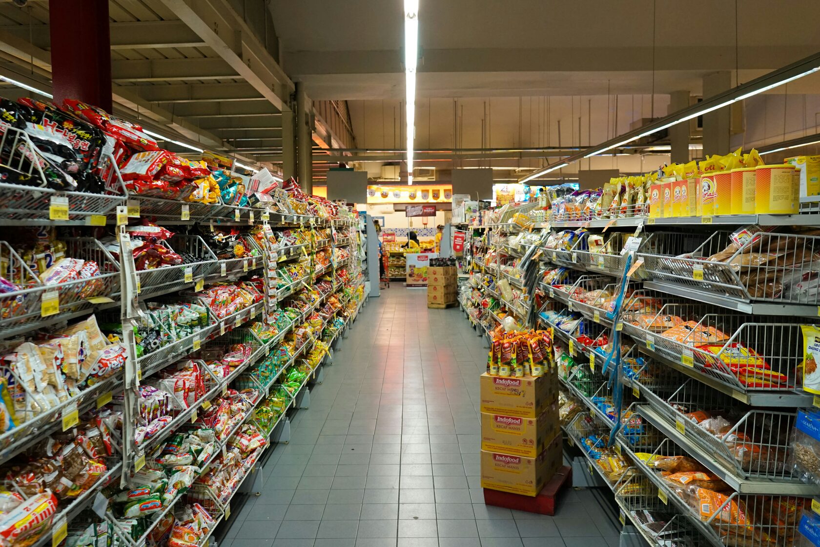
A typical photo with YOLO detections. And an example of a camera can be seen at bottom of the photo.

Pipeline v0 (embedder + search space) and v1 (v0 + realgram)

The very first solution, v0, consisted of an embedder and a search space:
  1. We crop regions based on YOLO detections.
  2. Each crop is passed through the embedder to obtain a vector representation.
  3. Search for the nearest vector in Qdrant, which stores the search space with embeddings and metadata of annotated crops.
  4. We take the top-1 result by cosine similarity and assign the product class.
The main drawback is that we only consider visual context and ignore spatial context. Nevertheless, even this simple approach achieved a classification metric of around 85%.
The v1 solution added realgram on top of the Qdrant search — an algorithm that takes into account what was present on the same shelf in recent annotations.
In short: for all products from the annotations, we compute an aging coefficient and a coordinate-overlap coefficient, combine them, and add the result to the cosine similarity from the v0 pipeline.

As a result, we obtain a more robust algorithm that incorporates more context and improves the metric up to 92%.

Remaining issues

Among the remaining issues:
  • The quality is still far from ideal: on difficult crops — where lighting is poor or part of the product is not visible — our predictions are still almost random, relying mainly on the shelf-level annotation context;
  • A large number of “flickers”: when, in consecutive images from the same camera, a product in a certain location has not changed, but its prediction changes due to volatility in the top of the search space. This is the main problem we will address in this article.

Object tracking

What object tracking is and why we need it in our task

At first glance, object tracking doesn’t seem to fit our problem well: we don’t work with video streams, but with snapshots. Let’s first clarify what it is, and then explain how it can be applied to our task.
Object tracking is the task of matching the same objects across different frames. In its classical form, it is solved on video streams with a high frame rate, where an object moves smoothly and the algorithm can rely on two types of signals:
  • visual features of the object;
  • its motion dynamics.
The main goal of tracking is to determine which object in the current frame corresponds to an object in the previous frame, even if it has slightly changed its position, scale, or appearance.

With or without visual descriptors?

There are two main approaches: tracking without visual descriptors and tracking with them.
The first category includes algorithms like SORT, which use only detections and a simple motion model (most often a Kalman filter). Such methods work well when changes between frames are small and the object can be predicted from its past trajectory. They are fast, lightweight, and well suited for real-time video streams.
When visual or temporal information is insufficient, methods with embeddings come into play, such as DeepSORT. Adding visual descriptors makes it possible to robustly match detections across frames even with long gaps, complex occlusions, or in situations where the motion model provides too little signal. In essence, the tracker compares objects not only by their coordinates but also by the “similarity” of their appearance.
An interesting challenge arises in tasks where frames appear infrequently—for example, once every few minutes or even every half hour. Under such conditions, standard motion models provide less useful signal, and visual features become the primary source of information.
Tracking then turns into a problem of matching independent snapshots with similar coordinates: we need to correctly link objects that may have slightly shifted, disappeared, or reappeared.
That’s why high-quality descriptors that are robust to changes in viewpoint, lighting, and object position become especially important.

Solution v2: v1 + tracking

Applying tracking to our task

We formulated the following hypothesis: in consecutive frames from the same camera, products at the same coordinates usually change only slightly. This is an averaged observation—dynamics vary across cameras: for example, in the dairy category, product movement is noticeably higher than in others.
Accordingly, if an object matches in coordinates and looks visually similar, it is highly likely to be the same product as in the previous frame. This means we can add to the pipeline an algorithm that compares coordinates and embeddings across neighboring images and obtain a kind of “lightweight tracking.”
This should:
  • increase prediction stability,
  • reduce the number of “flickers,”
  • potentially improve classification quality.
An example of how products change at the same coordinates across different frames is shown below.

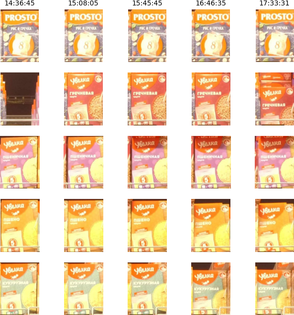
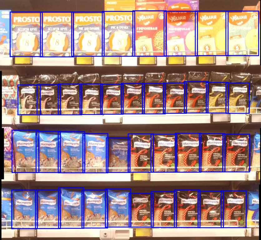
A column represents a single image from the camera, and a row represents one set of coordinates. On this particular camera, products hardly change over time and look almost identical, so tracking works well. However, things are far from this good on all cameras.

Modified DeepSORT

We didn’t want to reinvent the wheel when there are so many open-source tracking implementations available, so based on popularity and ease of integration, we chose the DeepSORT algorithm.
In the original DeepSORT, tracks (existing detections from previous frames) are first matched by embeddings (with preliminary filtering of unrealistic candidates based on coordinates), and then IoU-based matching is applied to the remaining detections.
In our case, this approach was not optimal for two reasons.
First, shelves often contain multiple identical products with almost identical embeddings, which makes it easy to match the wrong objects (for example, matching the first bottle of cola in one frame with the second bottle of cola in another).
Second, products generally move very little, while the requirements for matching reliability are quite high. As a result, separating IoU matching and embedding-based matching turned out to be inefficient—it is better to take both signals into account simultaneously.
We therefore adapted DeepSORT as follows: we first perform IoU-based matching, and only for detections that match by IoU do we additionally compute embedding-based matching. In this way, we combine the advantages of both approaches.
Of course, false matches did not disappear completely (for example, a bottle of sparkling water is replaced with still water → high IoU, high cosine similarity → high final score). Therefore, we increased the thresholds to match only truly confident pairs.
Below are block diagrams of the original DeepSORT (top) and the modified version (bottom).

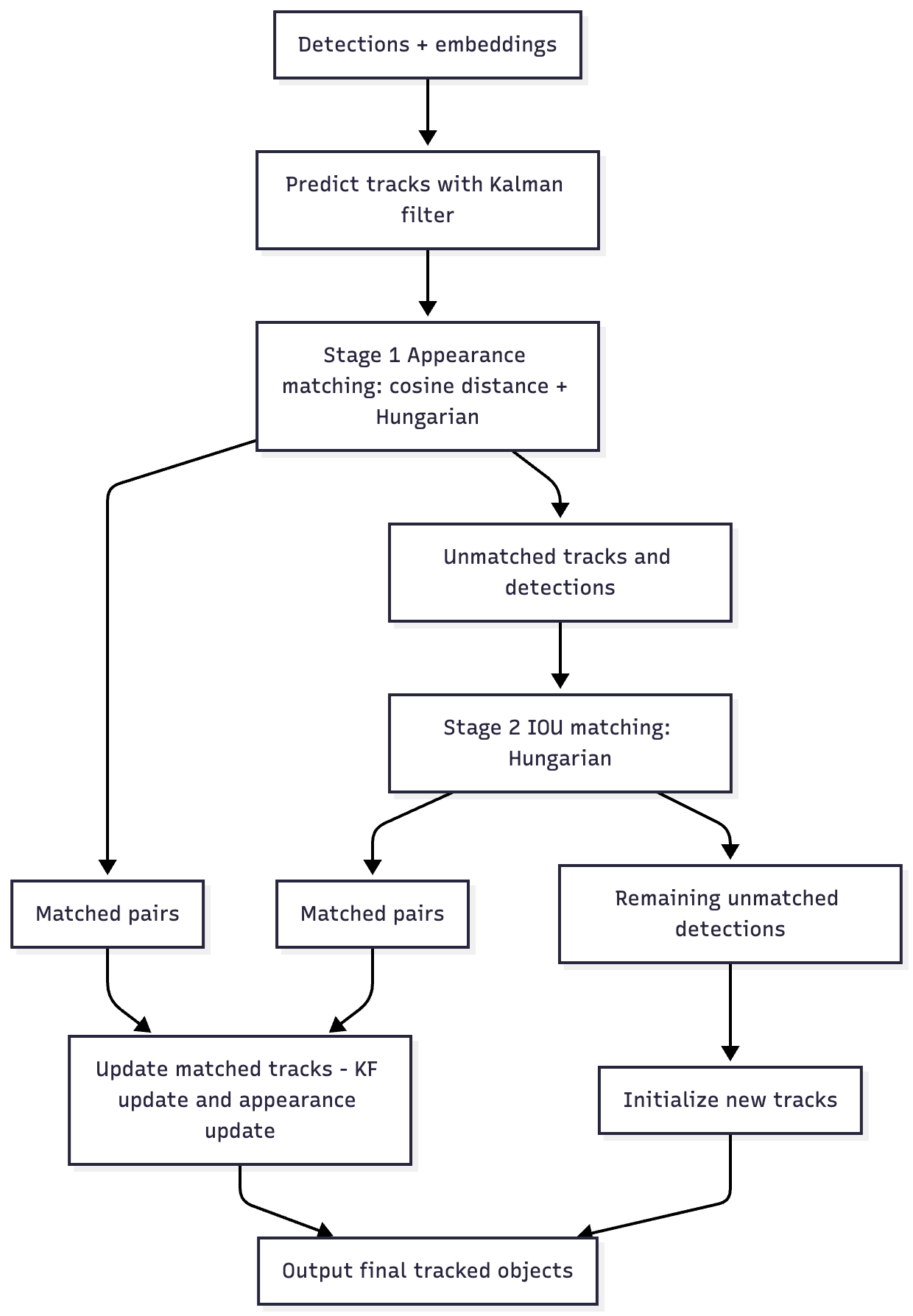
Original DeepSORT: first, matching by embeddings (filtering out unrealistic candidates using a Kalman filter), and then IoU-based matching for detections that were not matched by embeddings.

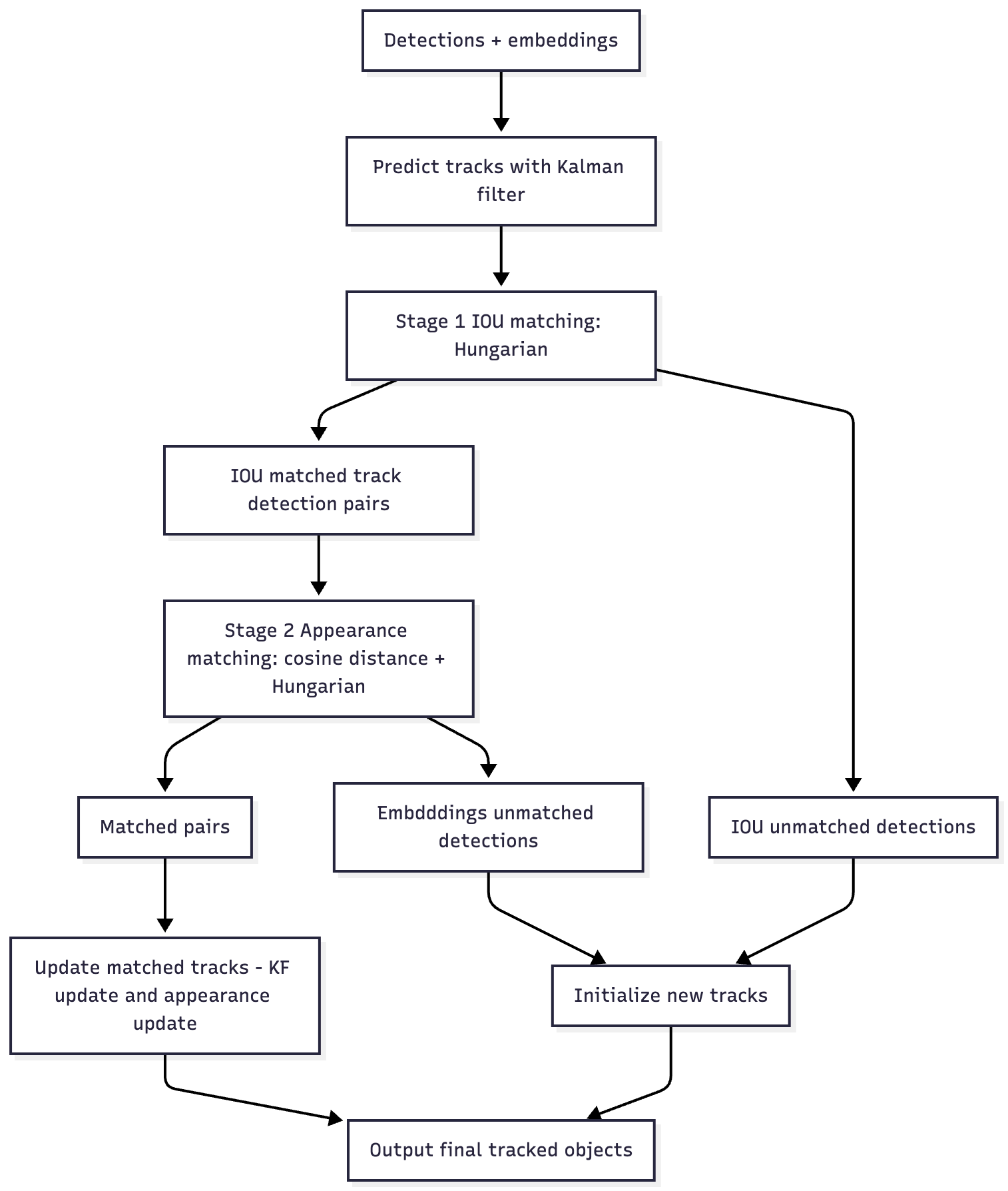
Our version of DeepSORT: first, IoU-based matching, and only for detections that were matched by IoU, embedding-based matching (since products in our case hardly move and visual descriptors are more important for us).

Pipeline v2: adding tracking

We keep the v1 pipeline unchanged: we build embeddings, query Qdrant for the nearest crops, compute realgram, and obtain an intermediate prediction.
At the next stage, we find the most recent unused annotation from this camera (each annotation is used only once) and perform tracking between detections on the annotated image and the current detections.
About the “most recent unused annotation”

Tracking across frames is a good idea, but if the source for tracking is just the pipeline’s prediction (with, say, 90% accuracy), then in 10% of cases the tracking will “propagate” the error further. To reduce this effect, we use annotations as a more reliable source.

For each frame, we check whether an annotation is available. When a new annotation appears, we run tracking from it once and then continue tracking on intermediate frames. Yes, with each frame the number of tracks created from annotations (we call them “anchor” tracks) decreases, but depending on the thresholds, between 20% and 50% of “anchor” tracks are preserved between annotations.
Next, a branching point appears in the pipeline:

  • If the tracking score (IoU between boxes × cosine similarity between embeddings) is higher than the intermediate prediction score minus a constant (a hyperparameter that defines the level of trust in tracking), we take the prediction from the previous frame.
  • Otherwise, we take the intermediate prediction and initialize a track with it.

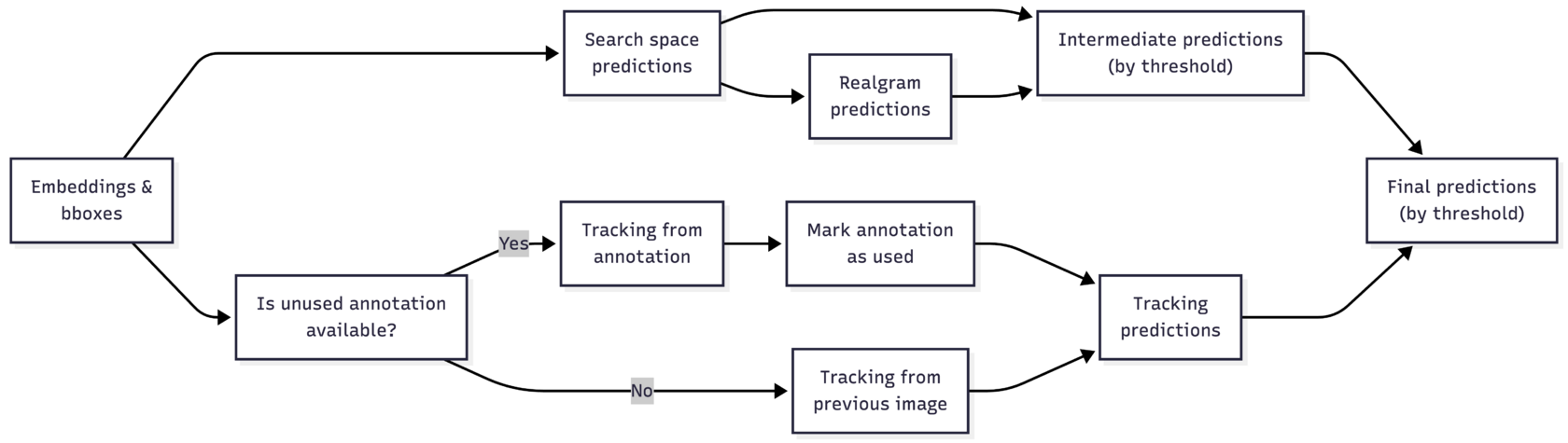
The v2 pipeline looks roughly as follows: we obtain intermediate predictions from the search space and realgram; obtain predictions from tracking; and then select between them based on a score with a threshold.

As we can see, in addition to a single hyperparameter for choosing between the intermediate prediction and the tracking result, the tracking itself introduces additional parameters (IoU threshold, IoU × cosine threshold, and others). As a result, the number of hyperparameters continues to grow.

Nevertheless, the result is there: the metric (its calculation method was described in the previous article) increased from 92% to 94%, and the number of “flickers” decreased roughly by half.

As for the “flicker” metric, at that time we had not yet introduced a separate formal metric, so the estimate of their reduction is qualitative in nature. However, the effect is easy to explain: after adding tracking, the prediction for the current frame is inherited from the previous one much more often, whereas previously neighboring frames were processed independently.

As a result, predictions across adjacent frames began to coincide significantly more frequently, which visually reduces the number of “flickers.”

Results

We continued to develop the baseline with the embedder and realgram and added tracking. As a result, quality improved from 92% to 94%, and predictions became noticeably more stable: the number of “flickers” decreased by about 50%.
However, version v2 still has significant issues:
  • Growth in the number of hyperparameters. Realgram had around 10 hyperparameters, and tracking added about 5 more. Even Optuna stopped handling the search effectively, and the risk of overfitting increased, since parameter tuning is performed each time on a limited dataset.
  • False positives in tracking. Even with a high tracking score, tracking can “propagate” incorrect predictions. For example, at the same coordinates, one product may be replaced by another flavor or variant that is visually almost indistinguishable. In such cases, the tracker easily picks up the wrong class.
  • Increased complexity of candidate selection. With the addition of tracking, we further complicated the selection problem: now we have many candidates from the top search space, realgram, and tracking. There may be one candidate, or there may be twenty. How should we choose among them?
Some of these limitations are addressed by adding a second-level classifier. That is exactly what we will discuss in our next article.
Huge thanks to our CV engineers, Oleksandr Korotaievskyi and Artem Smetanin, for preparing this material and sharing their experience with us.
AI Computer Vision