
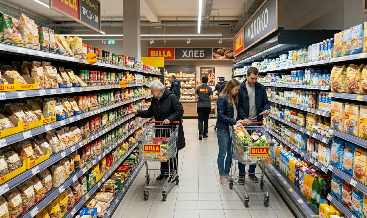
This is the third part of our series on retail product classification. The previous articles — part 1 and part 2 — are worth reading first so you don't get lost. Here's a quick recap to refresh your memory.
Recap
The Task
Our goal is to identify products on each shelf using photos from cameras mounted in supermarkets. This feeds into analytics, out-of-stock detection, and improving on-shelf availability. Every few days, one photo from each camera goes through manual annotation. Here's an example of what the camera captures:
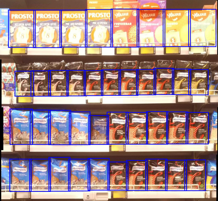
A typical camera photo with YOLO detections (and a typical shot of the camera itself below)
Pipelines v0–v2
v0 (embedder + search space) The very first solution, v0, combined an embedder with a search space: we crop the bounding boxes from YOLO detections, run each crop through the embedder to get an embedding, query Qdrant — where we store embeddings and metadata for annotated crops — and pick the top-1 result by cosine similarity to get the product class. The major downside was that it only used visual context with no spatial awareness. Even so, this simple approach achieved around 85% classification accuracy.
v1 (v0 + realgram) v1 layered realgram on top of the Qdrant search — an algorithm that takes into account what appeared on the same shelf in recent annotations. In short: for every product in an annotation, we compute a staleness coefficient and a coordinate overlap coefficient, combine them, and add the result to the cosine similarity from v0. This produced a more robust algorithm with richer context, pushing the metric up to 92%.
v2 (v1 + tracking) v2 introduced inter-frame tracking via a modified DeepSORT algorithm: we compare detections on adjacent frames first by IoU, then apply cosine similarity between embeddings on the IoU-matched pairs; if the score is high enough, we carry the prediction forward from the previous frame. This lifted the metric from 92% to 94% and noticeably reduced "flickering" — cases where the product doesn't change between adjacent frames, but the predictions jump around.
Remaining Problems
A few issues remained:
- Too many hyperparameters — roughly 15 across the full pipeline. You can tune them manually (painful) or with Optuna, but risk overfitting since you're always tuning on a specific dataset.
- Too many candidates — for each crop, the search space, realgram, and tracking can together produce up to 20 candidates. Picking the right one is tricky when several candidates have high scores — and comparing those scores directly is hard, since they come from different sources: cosine similarity for the embedder, cosine similarity + extra coefficients for realgram, and IoU × cosine similarity for tracking.
Ideally, we'd have an algorithm that takes all possible candidates and all possible features as input, and decides which product is correct. Fortunately, such an algorithm exists — but first, let's talk about what other features we could use to inform that decision.
Contextual Features
What we're already using
Here's a rundown of the signals that currently influence predictions in pipeline v2:
- Search space — from the top-20 nearest crops, we use the maximum cosine similarity per unique product.
- Realgram — for each unique candidate, the maximum score (cosine similarity + staleness/overlap coefficients).
- Tracking — the final score (IoU × cosine similarity).
What else could we use?
Below is a summary of the feature types we considered when building the pipeline, and how they ended up being used. This isn't a universal recommendation — different setups will benefit from different signals. The goal here is to document the solution space and the outcomes of our feature selection experiments.
Trying to account for all of these signals manually would be a nightmare. But since all these features are numeric (or binary/categorical — which is also numeric, essentially), we can tackle this as a classic tabular ML problem.
Solution v3: v2 + Second-Stage Classifier
Classification vs. ranking
At first glance, "pick the right class out of N candidates" sounds like a binary classification problem. But we hit an immediate snag: the number of candidates varies significantly across crops, which makes standard classification awkward — you'd need a fixed number of classes (or artificially cap candidates at 2–3, which raises its own questions). A better framing is ranking with a binary target: among an arbitrary number of candidates, exactly one is correct and the rest are not. This narrows the toolset, but fits our problem perfectly.
CatBoostRanker
Most popular open-source tabular libraries support ranking — LightGBM, XGBoost, CatBoost. We went with CatBoost: it has the widest selection of ranking loss functions and metrics, the whole team was already familiar with it, and it's always been a reliable baseline.
There's a great CatBoost ranking tutorial that covers the different loss functions. We concluded that QuerySoftMax was the right fit for our task. In typical ranking tasks there's no single correct answer — just a correctly ordered list of candidates. In our case, though, it's binary: one candidate is right, all others are wrong. QuerySoftMax handles this well — it's essentially standard softmax + cross-entropy, but computed separately within each group and then normalized by group size. In our setup, one group = one crop, and all candidates from the search space, realgram, and tracking form the ranking group with a binary target.
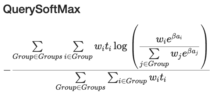
We compute the familiar softmax + cross-entropy across all groups and sum them up, with normalization by group size to account for the fact that groups can vary a lot. (Source)
Training CatBoostRanker is pretty straightforward — the parameters are mostly the same as for a standard boosting classifier (depth, learning rate, regularization, and so on), Optuna works just as well for hyperparameter tuning, and GPU training is supported. We started with around 100 features and, with the help of feature importance analysis and SHAP, trimmed that down to 36 features without a meaningful quality drop — while also factoring in implementation cost, since some features would have required scanning the entire search space (slow and expensive), while others could simply be pulled from the database.
Pipeline v3: adding CatBoost on top of everything
We kept the v2 pipeline entirely intact — search space, realgram, and tracking — but this time extracted all the auxiliary features described above from each of them. On top of those, we added size, annotation, and category features, and assembled for each crop an N × M table (N = number of candidates, which varies per crop; M = number of features, 36 in the first model). This table goes into CatBoost, which outputs logits for all candidates. Within a group you can convert those to probabilities, but there's no real need — we just take the top-1.


This crop has 3 candidates. The table shows some of the features for this crop (base = search space features, rg = realgram features, tr = tracking features), plus the CatBoost logits in the last column — which we use to select the top-1.
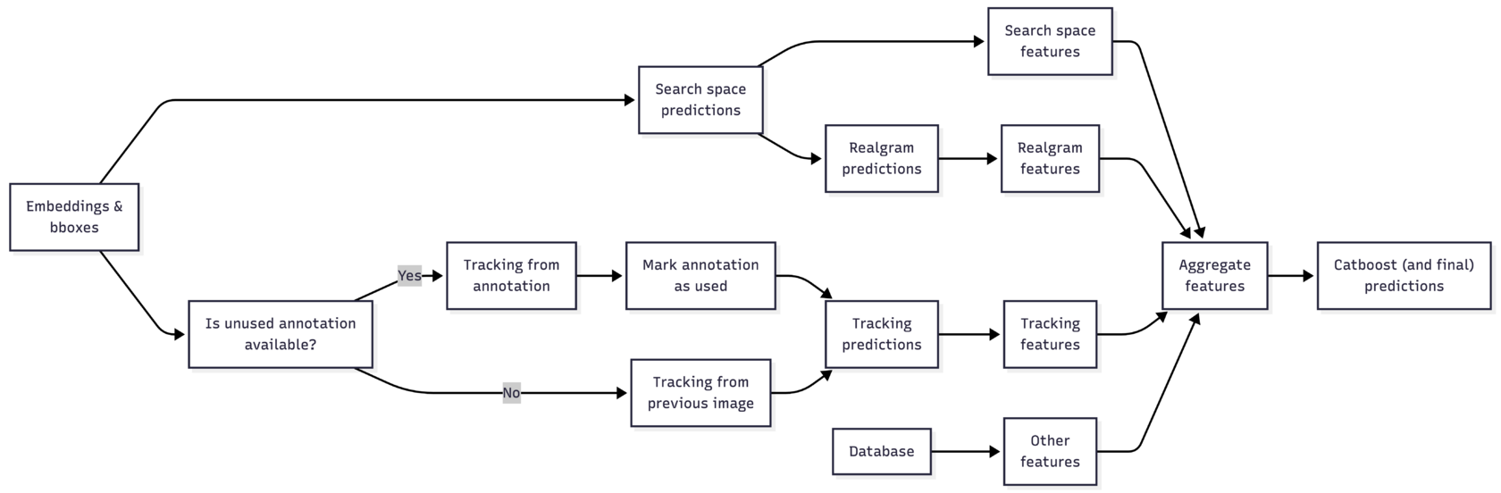
Pipeline v3: we pull features from the search space, realgram, tracking, and the database, aggregate them, and feed everything into a second-stage model.
Beyond pushing the metric from 94% to 96%, this approach opened up a whole Pandora's box of experiments — we could now try all kinds of new features (most of which, frankly, didn't move the needle, but still).
Pipeline v3.1: adding anti-flickering features
For a while we ran CatBoost with 36 features, tried new signals, collected new datasets — but the metric wouldn't budge. Then we noticed that flickering was back. Why? Because in the old pipeline, tracking almost always made the final call by simply carrying the prediction from the previous frame forward. Now, tracking was just one of many features, and CatBoost was weighing everything together — which meant it no longer had that built-in temporal consistency.
Examples of flickering at the same coordinates on consecutive photos:
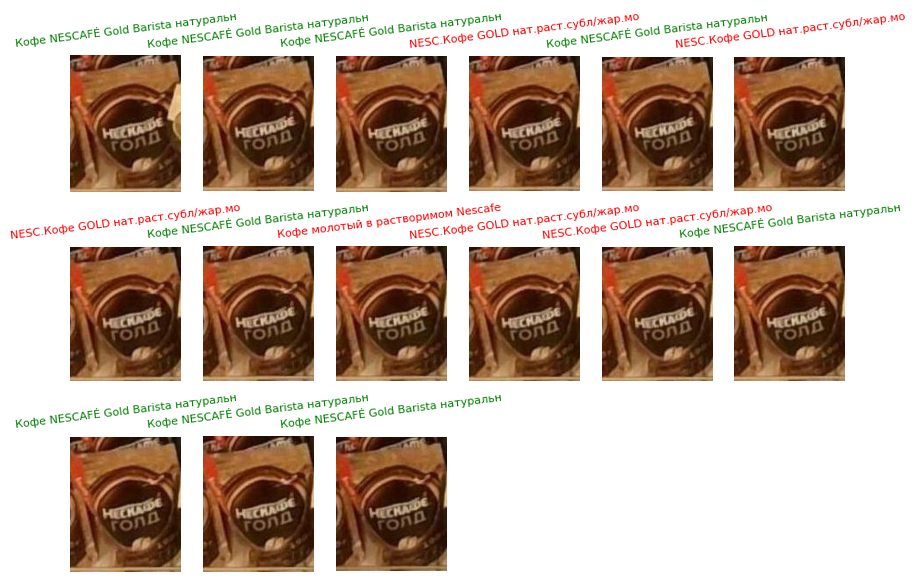
The product doesn't change at all, but predictions flip back and forth between two classes.
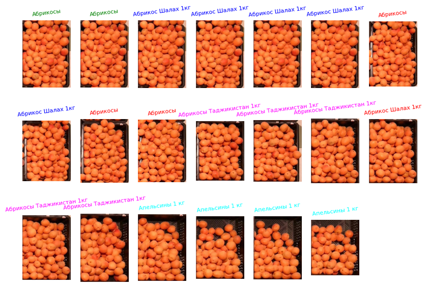
Apricots magically turn into oranges.
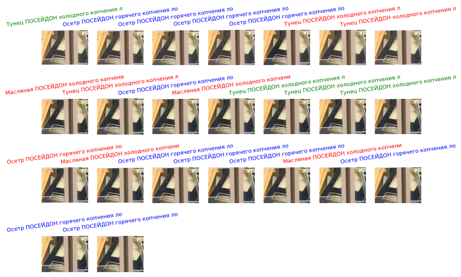
Tuna, sturgeon, or butterfish? You have 30 seconds.
What we wanted: fewer flickers, but without just blindly carrying predictions forward (which would hurt quality). The solution was a set of 13 new features (bringing the total to 49) computed from predictions at the same coordinates across the previous N frames from that camera. A few examples:
- Was this candidate predicted at these coordinates in the previous frame? The previous 3? The previous 5?
- How many products (unique / total) have been predicted at these coordinates over the previous N frames?
- Is this candidate the most frequently predicted one at these coordinates over the previous N frames?
These features worked — they didn't hurt quality (which was the top priority), and reduced flickering by 40% compared to CatBoost without them, bringing it roughly back to the level we had in v2 before CatBoost was introduced.
What didn't work?
Over the course of the project we probably tried a few hundred different features. Most didn't help, but after each failed experiment we tried to understand why. A few notable examples:
Size features What we tried: crop size in pixels/meters, difference between crop size and DB product size, z-score between the current diff and historical diffs, and so on. Why they didn't help: qualitative analysis showed they were useful in specific cases (telling a 0.5L bottle from a 1.5L one, or 200g peas from 400g), but in most cases they just added noise — for products with multiple flavor/variety variants, size doesn't differentiate anything meaningful.
Price tag features What we tried: whether the nearest price tags were detected, the value of the nearest tag to the left/right, whether that value matched the DB price. Why they didn't help: OCR worked well enough, but not on every camera (lighting issues, image quality); DB prices weren't always updated to reflect discounts; and the correct price tag for a given product could be to the left, right, above, or below.
Embedding geometry features What we tried: whether the class centroid was the nearest to the crop's embedding, silhouette score from clustering all candidate embeddings for a given crop, and similar signals. Why they didn't help:however much we hoped ArcFace would cleanly separate embeddings, similar product classes still ended up with similar embeddings — and UMAP / t-SNE / PCA visualizations confirmed that many classes were nearly impossible to disentangle.
Results
We implemented a second-stage classifier (or, more precisely, ranker) that takes 49 features from a wide variety of sources and uses them to make a final prediction, lifting accuracy from 94% to 96%.
That's where the interesting implementation details of our pipeline end — for now. But as we all know, there's always more to do, so we wanted to take a closer look at those stubborn 4% of errors.
Error analysis showed that the majority are meta-errors outside our pipeline's control:
- Annotation errors — tricky cases where an annotator assigns a class similar to the correct one, affecting both the metric and the predictions (since they end up in the search space and CatBoost features).
- Displaced and knocked cameras — this resets realgram, which is one of the strongest signals, taking predictions down with it.
- New products — we simply can't predict these correctly since they don't exist in the search space or candidate pool yet. (We'll cover how we detect and fast-track these for annotation in a separate article.)
Building a pipeline this complex — with many details left out to keep things readable — and running a million different experiments took over a year. But we think the result is a solid and fairly robust system, and we hope this series helps anyone facing a similar challenge.
Huge thanks to our engineers Aleksandr Korotaevskiy and Artem Smetanin for preparing this material and sharing their experience with us.

